DDIA Chapter 6: Partitioning

DDIA series: Chapter 6 - Partitioning Part 2: Distributed Data

Partitioning is the process of dividing the main database into smaller chunks (databases on their own). These smaller chunks are separated instances, each of them having its own CPU, RAM, and Disk space.

The main reason to partition the data is simply scalability. The partition can be placed on different nodes (servers) in different geo-locations to reduce latency for a specific set of users.

Each partition can have its own replicas, as all of the pros and cons that come with them apply from the previous chapter.

Partitioning and Replication#

As I said, partitioning in most cases is combined with replication. Copies are stored for each partition on multiple nodes. A node can store more than one partition.

Partitioning helps us scale horizontally, because instead of storing the entire dataset on one machine, we distribute it across many. Replication then ensures that if one node fails, another copy of the same partition is still available.

When partitioning is combined with leader-based replication, each partition has its own leader and its own set of followers.

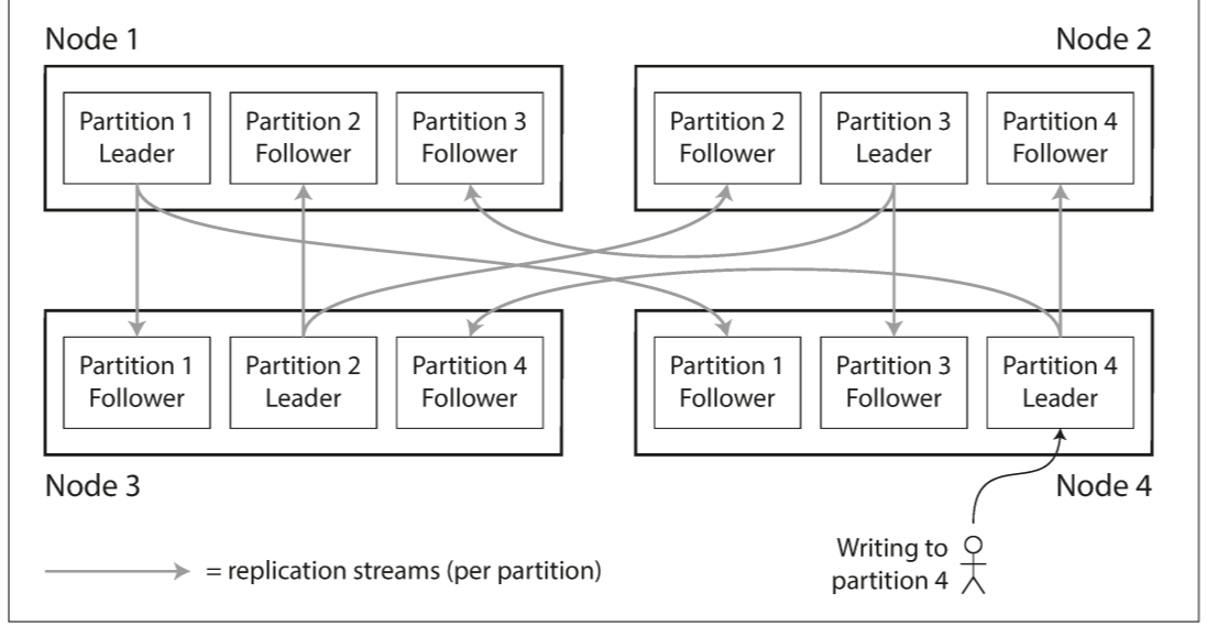
Each partition has its own leader and followers. A node can be a leader for one partition and a follower for another.

Partitioning of Key-Value Data#

A common question arises when we decide to partition our data:

• How do we decide which rows/records to store on which nodes?

The goal is to distribute the data evenly across the nodes, so we can optimize bandwidth and avoid overloading a single machine.

An unfair distribution leads to so-called hot spots. These are partitions that handle disproportionately higher loads compared to others.

To avoid them, we could randomly place records on nodes. However, another problem arises: how do we know which node holds which data? This would force us to query all partitions for a single record, which completely defeats the purpose of partitioning.

A better approach is to use a key-value data model.

Let’s assume we always access a record by its primary key. For example (from the book), in an old-fashioned paper encyclopedia, entries are sorted alphabetically by title. If you want to find a topic, you go directly to the section that corresponds to its first letter; you don’t scan the entire book.

Similarly, in a distributed database, we can partition data based on the key. Instead of random placement, we derive the partition directly from the key itself. That way, given a key, we can deterministically know which partition (and therefore which node) holds the data without querying every node.

Partitioning by Key Range#

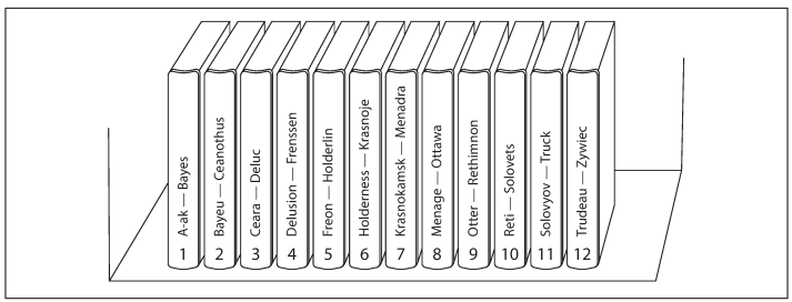
Another way to partition data is by assigning key ranges to each partition. Each range covers a continuous set of keys, and when a user wants to query a record, you can easily determine which partition contains that key.

The key ranges do not have to be evenly spaced. Some ranges may naturally contain more keys than others. For example, one partition might cover popular keys and become much larger than another partition that rarely has keys. This imbalance can lead to hot spots, where one partition experiences heavy load while others sit mostly idle.

To avoid this, the partition boundaries should adapt to the data. They can be chosen manually by an administrator, or automatically by the database system, which can adjust ranges as the dataset grows or changes.

Within each partition, keys can be kept in sorted order. This makes range queries efficient: you can fetch all keys within a certain range without scanning the entire partition.

However, key-range partitioning can create new hot spots depending on the access pattern. Using the timestamp as the first element of the key means all writes for “today” go to the same partition, overloading it while older partitions sit idle. A common solution is to prefix the key with another value, like the sensor ID, so partitions are distributed across both the sensor and the time range. This spreads the write load more evenly, though range queries across multiple sensors now require separate queries per sensor.

Partitioning by Hash of Key#

Another approach to partitioning is to use a hash function. We pass a value such as a timestamp, user ID, or key through the hash function to generate a hash ID, then assign the partition based on the range in which the hash falls. This ensures that keys are distributed evenly across partitions, reducing the risk of hot spots.

A good hash function spreads skewed data uniformly. For example, a 32-bit hash function takes a string and returns a random number between 0 and 2³² − 1. Even similar input keys produce very different hashes, which helps balance the load across partitions.

Many databases use standard hash functions like MD5 (Cassandra, MongoDB) or Fowler–Noll–Vo (Voldemort). Simple built-in hash functions in programming languages may not be suitable, because they can produce inconsistent values across different processes. (from the book)

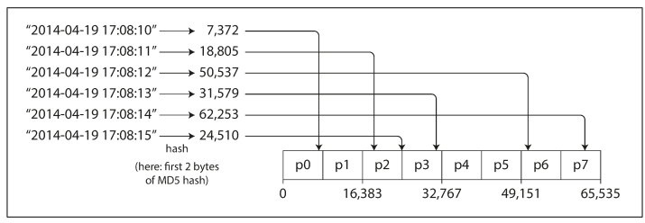
Once keys are hashed, each partition is assigned a range of hash values rather than key values. Every key whose hash falls within that range is stored in the corresponding partition.

The main trade-off with hash partitioning is that it destroys key order. Keys that were adjacent in a key-range scheme are now scattered, so efficient range queries are no longer possible.

Partitioning and Secondary Indexes#

So far, we have looked over types of partitioning that are based on the key-value data model. This means we can determine partitions only for records that are accessed using the primary key. However, when secondary index is used we are no longer able to find the correct partition because the index itself was not used in the partitioning logic (it’s not used to identify the user).

There are two types of partitions when it comes to secondary indexes.

Indexes by Document#

Each partition maintains its own indexes for the documents it contains, so writes only affect the relevant partition. However, reading from a secondary index may require querying all partitions and combining the results, an approach known as scatter/gather. This can be expensive and prone to tail latency, though it is widely used in databases like MongoDB, Cassandra, and Elasticsearch. Ideally, partitioning should be structured so that secondary index queries can be served from a single partition, but this is not always possible.

Indexes by Term#

Global, or term-partitioned, secondary indexes cover data across all partitions rather than being local to each partition. The index itself is also partitioned either by term or by a hash of the term to avoid bottlenecks and distribute load evenly.

This approach makes reads more efficient, because a client can query only the partition containing the desired term instead of performing scatter/gather across all partitions. The downside is that writes are more complex and slower, since updating a single document may require changes across multiple index partitions.

Rebalancing Partitions#

Sometimes we need to move data between partitions, for example, when adding more hardware or replacing a failed machine. This process is called rebalancing partitions. It applies regardless of whether you’re using key-range or hash-based partitioning.

---

Hash mod N#

Using hash mod N is stupid. A key’s hash is modulo the number of partitions, which sounds simple, but it has a big flaw. Anytime a partition is added or removed, every key has to be rehashed to determine its new partition. This means almost all data must move, which is extremely inefficient. This is exactly why consistent hashing was invented: it minimizes the amount of data that needs to be relocated when partitions change.

Fixed number of partitions#

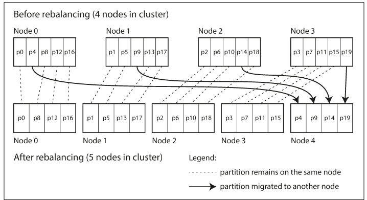
In this approach, we create many partitions upfront, for example, 1000 partitions for 10 nodes, and assign roughly 100 partitions to each node.

When we add a new node, we can “steal” some partitions from the existing nodes and assign them to the newcomer. The keys themselves don’t move; only the ownership of partitions changes. This avoids re-hashing or moving all data.

For example, imagine a system with 4 nodes, each holding 5 partitions. When a fifth node is added, one partition from each existing node can be reassigned to the new node, balancing the load across all nodes. The reassignment takes some time, but it preserves the original key-to-partition mapping.

Dynamic partitioning#

In dynamic partitioning, a partition is automatically split into two when it exceeds a certain size (for example, a memory or data threshold). If a large amount of data is deleted, partitions can also be merged. This approach works particularly well with key-range partitioning, where boundaries can adapt as data grows.

After a split, one of the new partitions can be moved to another node to maintain a balanced data distribution across the cluster.

This approach is practical because the number of partitions scales with the amount of data: more data leads to more partitions, and less data leads to fewer partitions.

However, there is an important caveat. When the database is empty or very small, it may start with only one partition, since no threshold has been exceeded yet. That means a single node will initially handle all reads and writes, which can create a bottleneck.

One way to mitigate this is to pre-split partitions in advance, based on expected key ranges. However, this only works well if you have a good understanding of the future key distribution.

Request Routing#

---

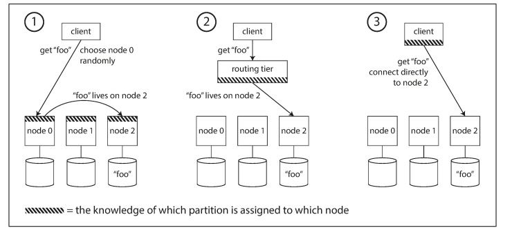
There is another way where we are using some key-value storage to store the key-ranges and their partition/node and IP addresses.

So far, we have partitioned the data and distributed partitions across multiple nodes. However, we still need a way to route each client request to the node that actually holds the relevant partition.

When rebalancing happens, partition-to-node assignments change. Without a mechanism to track these changes and redirect requests accordingly, users would not be able to access their data.

For this, we need service discovery. This concept is not specific to databases—it is used in many distributed systems whenever we need to map a request to the correct service instance.

There are several common approaches:

• A client sends a request to any node. If that node owns the partition, it handles the request; otherwise, it forwards the request to the correct node.
• Clients send all requests to a separate routing tier (middleware). The router knows the current partition-to-node mapping and forwards the request to the appropriate node.
• Clients are aware of the partition-to-node assignment and connect directly to the correct node without an intermediate layer.

---

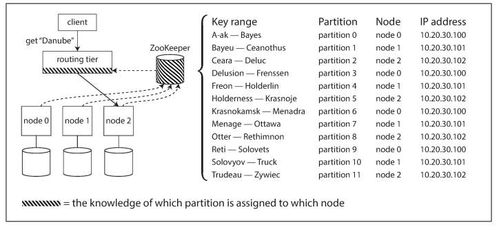
Another approach (the second one) is to maintain a small distributed key-value store that tracks partition ranges, their assigned nodes, and their network addresses. This metadata service is then queried to determine where a request should be routed.

Summary#

In this chapter, the author explains how to partition a large dataset into smaller subsets when a single machine is no longer sufficient. The main goal is to distribute both data and query load evenly across nodes and avoid hot spots.

Two primary partitioning strategies are discussed: key-range partitioning, which preserves ordering and supports efficient range queries but risks hot spots, and hash partitioning, which distributes load more evenly but loses key ordering.

The chapter also explores rebalancing strategies, dynamic vs fixed partitions, and hybrid approaches. Additionally, it explains how secondary indexes interact with partitioning (local vs global indexes) and how request routing ensures clients can reach the correct partition.

Overall, partitioning enables horizontal scalability, but operations that span multiple partitions introduce additional complexity.