DDIA Chapter 3: Storage and Retrieval

DDIA series: Chapter 3 - Storage and Retrieval Part 1: Foundations of Data Systems

There are two operations that the database, on a very high-level should support.

• Storing the data that is being written.
• Retrieving the data when it’s being read.

At the beginning of the chapter the authors show an example of the simple implementation of both of these operations using simple bash scripts.

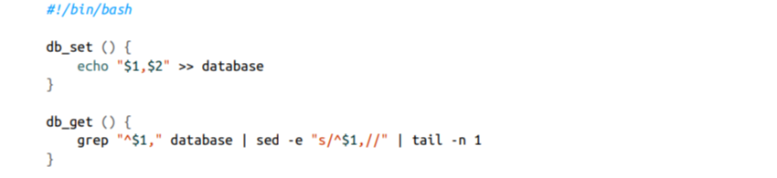
This is a simple implementation of a key-value-based store.

• The db_set method is used to store the input from the standard input to a location “database.”
  • The input comes as a key value for the first and second arguments.
• The db_get method is used to retrieve a value based on an argument key.

The storage format is very simple; it’s a comma-separated key-value pair. Every write appends to the end of the file, and every read finds the key by sequential scan. Reads should start from the end, as this implementation does not modify records; it appends the updated values to the end of the file, so we have to read from the end to ensure that the found key is most up-to-date.

The overall performance for write is quite good because appending to the end of the file it’s fast and easy operation.

Reads, on the other hand, will become a huge bottleneck when the records in this “database” become a lot. The main performance issues are coming from the sequential read, basically we don’t have an efficient way of searching for information.

To overcome these issues, production-ready databases have the concept of indexing. This is a different data structure used to store the information, which allows a very performant way of searching in most of the cases in 0(logn) operations.

Hash Indexes#

A hash index is an in-memory data structure that maps each key to a byte offset in an append-only data file. The data file itself is a log: new key–value pairs are always appended, never modified in place.

Whenever a new record is written:

• The key–value pair is appended to the log file.
• The in-memory hash map is updated to point the key to the new byte offset.

When a value is read:

• The hash map is used to find the byte offset.
• The system seeks directly to that position in the file and reads the value.

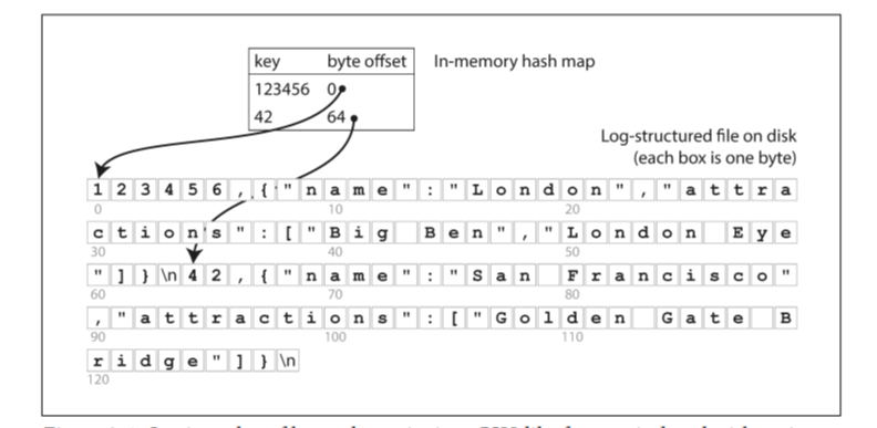
                    **(Figure 3-1 from the book, page 72)**

As we can see in the figure, each segment stores the key and the byte offset from which the algorithm can start reading the key and value within the file. This is very efficient for fast lookups, as it is O(1) time complexity of the operation.

However, to be able to use this index, we have to ensure that all of the segments can be stored within in-memory, as this is our only way to later read from the log file. The values themselves can be stored on disk and later pulled into memory for reads.

Since this structure is append-only, disallowing modification of data entries, we have to use a compaction algorithm to:

• Reduce the size of the segments, thus storing more of them in-memory.
• Remove duplicates of key-value pairs.
• Reduce the size of the stored data on disk.

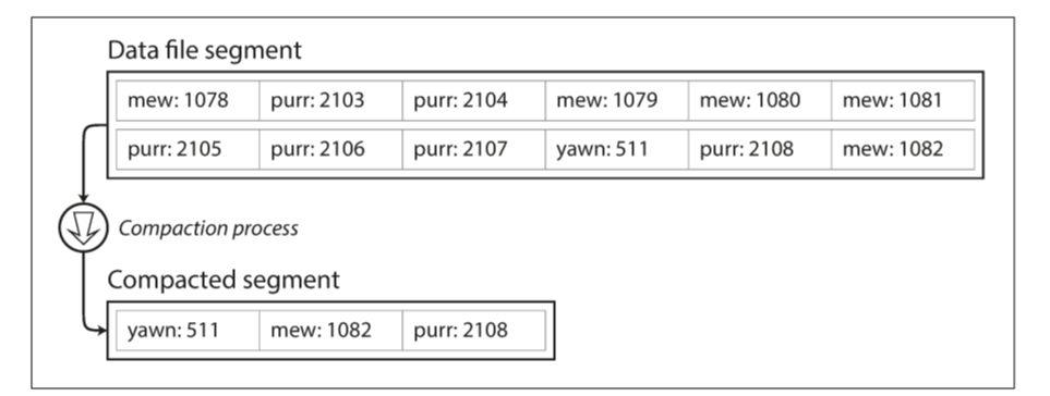
This compaction process is happening in the background by another process. It “freezes” the segment that is going to be compacted, thus creating a new one for newer writes in-memory. The newly created segment is written to a new file. While that process is happening, reads and write ops are happening using the old segment files. Old segments are deleted after the compaction process finishes.

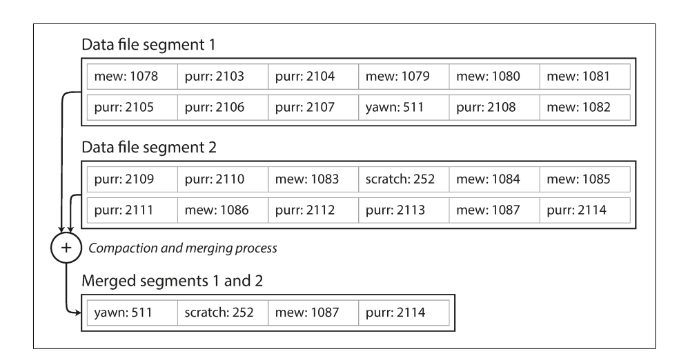
At any point in time, multiple segments may exist, each with its own hash map.

When compacting multiple segments:

• If the same key appears in multiple segments, the value from the newest segment is retained.

• If a key appears multiple times within a single segment, the last occurrence (the most recent write) is kept.

Notes:

• If the database is restarted, all of the hash-maps stored in memory are lost. This is quite bad because to restore the hash maps, we have to go over the log files and read the entirety of them from the beginning to the end, and pair the offset of the most up-to-date value for every key.
• Range queries are not supported because we cannot scan over all keys between related strings; we have to look up each key individually in the hash maps.

SSTables and LSM-Trees#

SSTables follow the same general idea as the append-only log structure described earlier, with segments written to disk and later compacted in the background. The difference is in how the data inside each segment is organized.

Instead of storing key-value pairs in the order in which they were written, SSTables store them sorted by key.

Because keys are stored in sorted order on disk, the database no longer needs a full in-memory map of every key. Instead, it can keep a much smaller, sparse index that maps key ranges to file offsets and use sequential disk reads to locate data efficiently.

Writes are still fast because data is not written directly into sorted files on disk.

Writes are first collected in an in-memory structure that maintains keys in sorted order. Once this structure reaches a certain size, it is flushed to disk as a new immutable SSTable. From that point on, the file is never modified.

Compaction in SSTables is conceptually similar to the compaction process described for log-segments, but it becomes more structured. Since SSTables are sorted, compaction works by merging multiple sorted files together, much like the merge step in merge sort. When the same key appears in multiple SSTables, the most recent value is kept, and older versions are discarded. Over time, this reduces disk usage and keeps read performance predictable.

LSM tree isn’t always a “tree” in the traditional sense; it can use skip lists, sorted arrays, or other in-memory structures, but the key idea is the same:

• keep recent writes in memory, flush them to disk as sorted files, and periodically merge (compact) those files to maintain efficiency.

Compaction in SSTables works by merging multiple sorted files, much like the merge step in merge sort. When the same key appears in multiple SSTables, the most recent value is kept, and older versions are discarded. Over time, this reduces disk usage and keeps read performance predictable.

B-Trees#

B-trees are one of the most widely used data structures in database engines. Like SSTables, they keep key-value pairs sorted by key, which allows fast lookups and efficient range queries, but that’s where the similarity ends.

Each node (or block/page) in a B-tree has a fixed size, often matching the size of a memory page (traditionally 4 KB). This design ensures that when a block is read from disk, the entire page is loaded into memory, minimizing disk I/O and keeping reads performant.

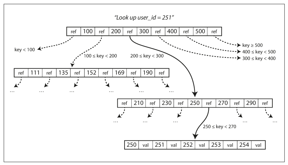
Each page has an address or pointer that can reference other pages on disk. The B-tree has a root page, and each child page stores a range of keys. When traversing the tree, binary search is typically used within a page to locate the correct key or child pointer. Leaf nodes either store the actual values or pointers to the locations of the values.

To modify a value, the corresponding page is loaded into memory, updated, and then written back to disk.

To insert a new key, the tree is traversed to find the page where the key belongs. If the page has space, the key is added directly. If the page is full, it is split into two, and the parent node is updated to reflect the new child. This splitting may propagate up the tree if the parent itself becomes full, maintaining the B-tree’s balance.

The overriding of a page on disk with new data does not mean we are changing the location of the page in the tree.

Comparing B-Trees and LSM-Trees#

In general, LSM-trees tend to be faster for writes, while B-trees are often preferred for performant reads.

Advantages of LSM-trees:

• Can sustain higher write throughput because writes are sequential and append-only.
• Avoid overwriting pages on disk, reducing random writes compared to B-trees.

Downsides of LSM-trees:

• Compaction can interfere with ongoing reads/writes.
• At very high write throughput, compaction may lag behind incoming writes, increasing the number of unmerged segments and slowing reads.
• Multiple copies of the same key may exist in different SSTables.

Advantages of B-trees:

• Each key exists in exactly one place.
• Reads are predictable and usually faster for single-key lookups.
• Well-mature and battle-tested, with stable performance across workloads.

Overall, LSM-trees are better for write-heavy workloads and modern storage engines, while B-trees remain reliable for read-heavy workloads and applications requiring strong consistency.

Other Indexing Structure#

A primary key uniquely identifies one row in a relational table, or one document in a document database, or one vertex in a graph database.

In relation databases, we can have different kinds of secondary indexes.

Covering index This index stores, alongside the row identifier, some additional column data. This reduces disk seeks because if a query only needs columns stored in the index, the database can satisfy the query directly from the index without fetching the full row.

Clustered index A clustered index stores the entire row within the index. In MySQL, for example, the primary key is a clustered index, and all secondary indexes reference the primary key.

Multi-column index This index allows searching efficiently on multiple columns, often used in queries with multiple filtering conditions or for geospatial or multi-dimensional data.

Full-text search / Fuzzy search / Inverted index Full-text search allows finding words or phrases inside large text collections, such as documents, articles, or web pages. The underlying data structure is an inverted index, which maps each term to the list of documents (or positions) where it appears.

Transaction Processing or Analytics?#

Traditional OLTP (Online Transaction Processing) databases are optimized for interactive applications that insert, update, or look up a small number of records at a time using indexes. Basically, more reads than writes.

However, when databases are used for analytics, the access patterns are very different. Analytic queries typically scan millions of rows, read only a few columns per record, and calculate aggregates such as sums, counts, or averages. For example, queries like “total revenue per store in January” or “which products are often bought together” involve processing large datasets rather than individual transactions.

This analytic workload is called OLAP (Online Analytic Processing). Unlike OLTP, OLAP focuses on summarizing, aggregating, and exploring data interactively for business purposes. Because of these different access patterns, OLTP databases can struggle with performance when handling large-scale aggregation queries.

Data Warehouse#

Data Warehouse’s goal is to provide the same data in the transaction processing database, for business analytics and data science engineers to use without affecting the performance of the transaction database.

This happens either through a periodic data dump or a continuous stream of updates. In both cases, the data is transformed first before being loaded into the warehouse.

A big advantage of having a separate warehouse is that it can be optimized for analytic access patterns, especially since typical OLTP indexing engines don’t perform well in the case of analytic queries

Column-Oriented Storage#

Column-oriented storage is designed to improve performance for analytical queries, especially when dealing with millions of rows and aggregations on a small subset of columns. In traditional row-oriented databases, entire rows are stored contiguously on disk. This means that even if a query only needs a few columns, the database often has to read all the columns of every row into memory, which can be inefficient for large datasets.

In contrast, column-oriented databases store each column separately in contiguous memory or disk regions. This layout allows queries to read only the columns needed, scanning through large datasets much more efficiently.

Aggregations, such as sums, averages, or counts, become faster because the database can process a single column in bulk without touching unrelated data. Additionally, columnar storage improves compression, since values in the same column are usually of the same type and often similar, further reducing I/O and memory usage.

Overall, column-oriented storage is more commonly used within OLAP workloads where queries scan large amounts of data but only require a few columns, making analytics and aggregation operations highly performant.

In data warehouses, analytical queries often compute aggregates like SUM, COUNT, or AVG over millions of rows. Materialized views store the results of such queries on disk, making repeated calculations much faster than scanning the raw data each time.

Because a materialized view is essentially a snapshot, it must be recomputed when the underlying data changes. While databases can be configured to update views automatically, this can be an expensive operation and may become a bottleneck for other ongoing database operations, so it should be planned carefully.

Summary#

Storage engines can generally be categorized into two main types:

OLTP – optimized for transactional processing

• Uses indexes for fast, selective reads.
• Typically supports interactive, user-facing applications.
• Writes can be slowed down if many indexes must be updated.

OLAP / Data Warehouses – optimized for analytics

• Primarily used by data analysts or data scientists, not end users.
• Handles fewer queries than OLTP systems, but each query often scans and aggregates large volumes of data in a short time.
• Often uses column-oriented storage to read only relevant columns efficiently.
• Can leverage materialized views or data cubes to precompute aggregates and speed up repeated queries.